1.1. Overview of the Autonomous System - An Explanation
The Autonomous System describes the high level software running on the ACU enabling the vehicle to drive autonomously.
The Autonomous System runs inside a docker container on the ACU and is implemented in multiple, modular ROS packages.
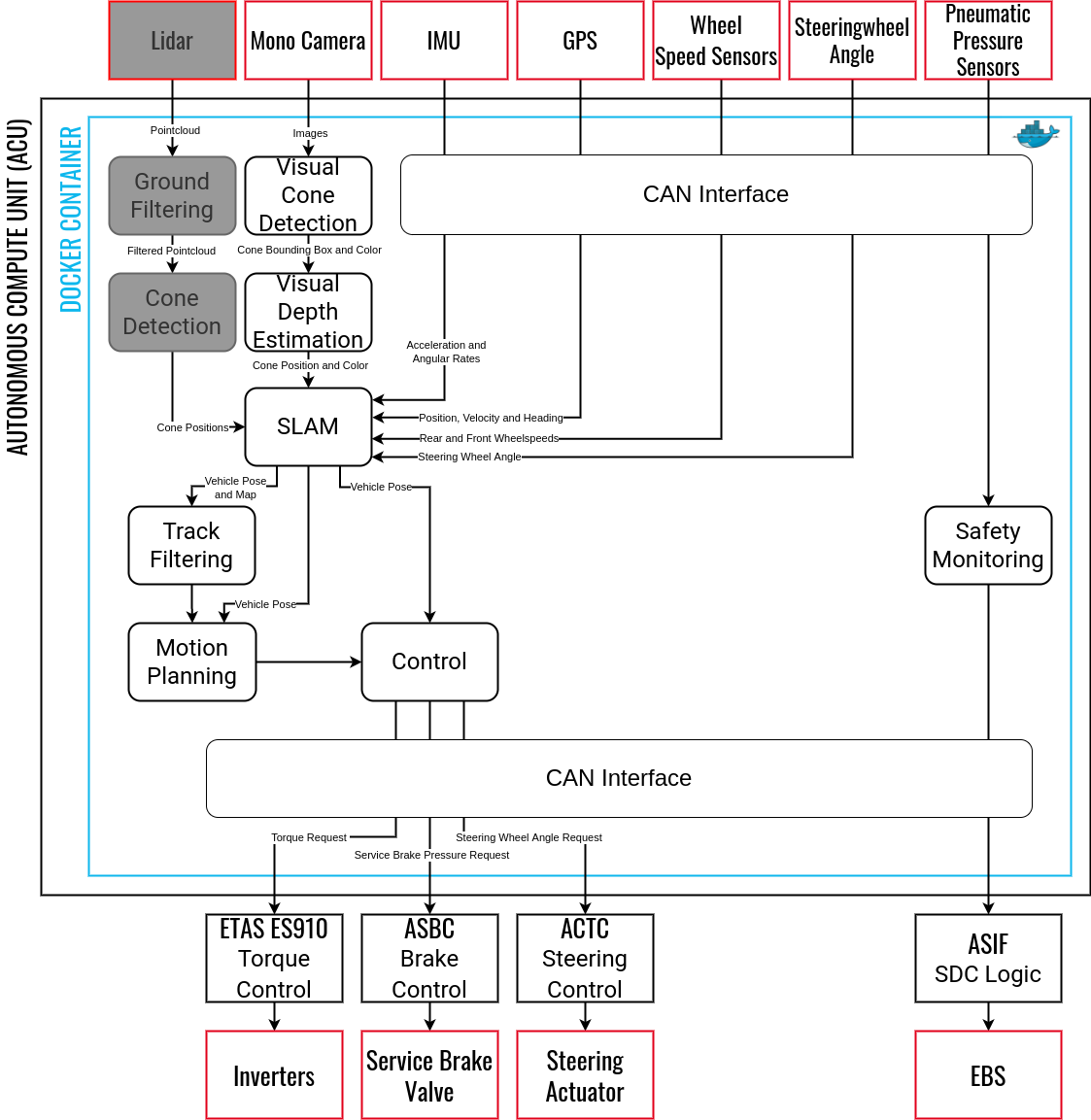
Fig. 1.1 Rough Overview of the Most Important Modules of the Autonomous System
Fig. 1.1 shows an overview of the Autonomous System and it’s most important module.
To enable the vehicle to drive autonomously the vehicle and thus the Autonomous System needs to know where the track is and where it should drive. The FSG Competition specifies for the track bounds (DE 6.2 in FSG Competition Handbook 22):
The track is marked with cones.
The left borders of the track are marked with small blue cones.
The right borders of the track are marked with small yellow cones.
Exit and entry lanes are marked with small orange cones
Big orange cones will be placed before and after start, finish and timekeeping lines
An example track layout for the acceleration discipline is shown in Fig. 1.2
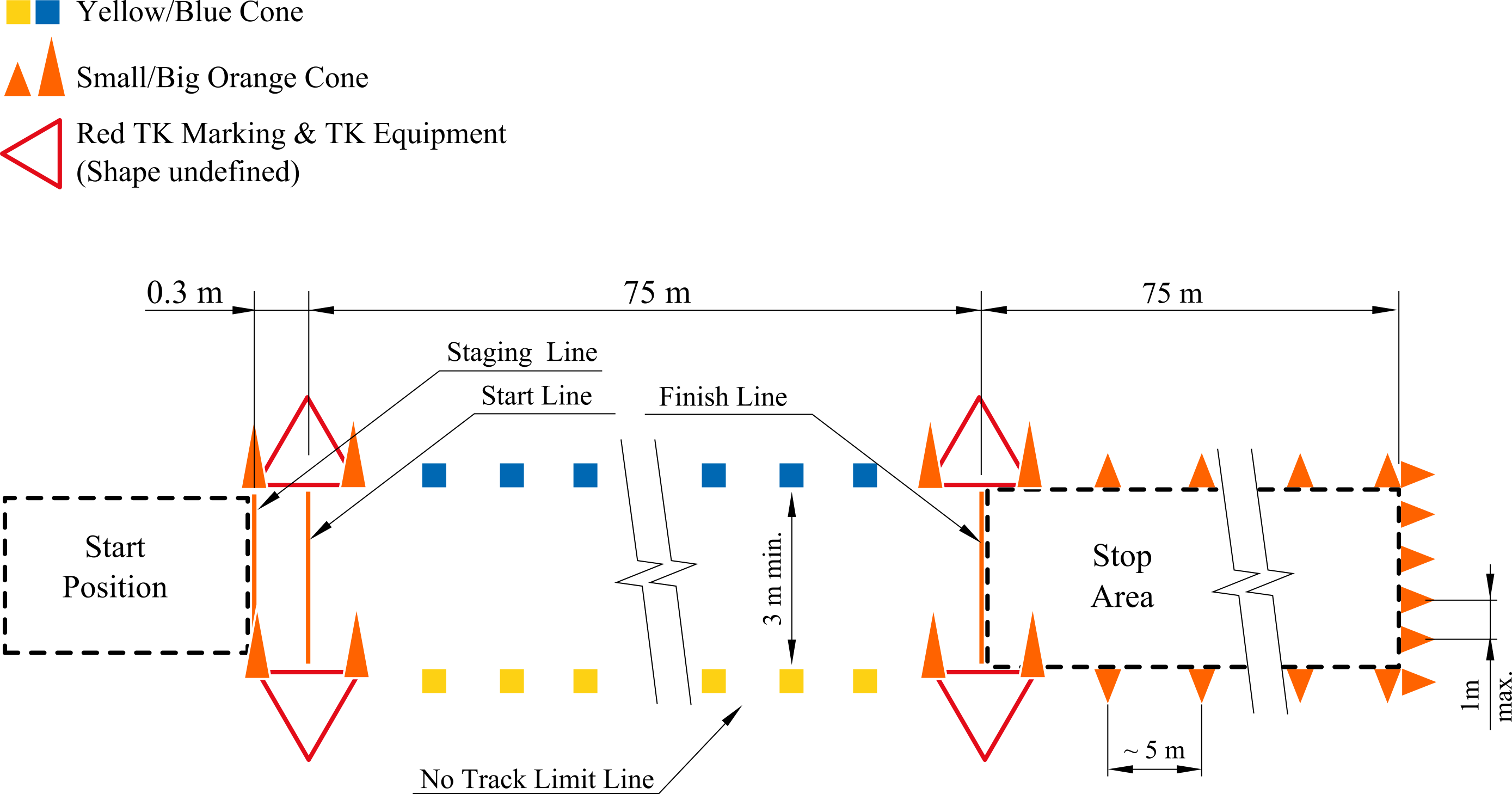
Fig. 1.2 Track Layout for DV Disciplines According to the Track Markings Specified in the FSG Competition Handbook
The FSG competition handbook specifies further:
No map data is provided by the officials.
Thus for disciplines where the maps are not previously known (Trackdrive and Autocross) the Autonomous System needs to perceive the cone positions to be able to know where the track is.
Even for disciplines where the maps are previously known (the FSG competition handbook precisely specifies the track layout of Skidpad and Acceleration) the Autonomous System still needs to perceive the trackbounds to align the known and preloaded map with the reality: A small deviation of 1 degree while staging the vehicle at the start position leads to a deviation of 1.3 m after 75 m, which is half of the 3 m track width.
The Autonomous System includes two modules for the perception of the trackbounds by perceiving the specified cones:
TRT Inference: a neural network based approach to perceive cones in camera images.
Lidar Perception: a approach based on the Himmelsbach algorithm for ground filtering and euclidian clustering for identifying cones in the remaining pointcloud.
Disclaimer: In the 2021/22 season (CM-22x: Emma) we already planned to also use the LIDAR perception. Since the perception range of the used LIDAR (Velodyne VLP-16) was only up to 8 m (because of the small number of channels) and limited development resources, we opted to only choose the TRT Inference.
Since the TRT Inference only outputs the location of the characteristic rectangle around the perceived cone and the vehicle needs to know the position of the cone relative to the vehicle, another module is used to calculate the position of the cone:
The Local Mapping module uses the intrinsic and extrinsic matrices of the camera to calculate the position of the cone relative to the vehicle based on the estimated tip of the cone.
In theory, the Autonomous System could plan it’s motion based on this output (this has also been done during the 2019/2021 season (CM-21x: Eva)). This proposal has multiple major drawbacks:
It is hard to compensate the distance the vehicle drove during the execution of the pipeline since this can be up to 200/400 ms (depending on the host machine)
The vehicle can only plan as far as it can currently see:
For the TRT Inference the perception range is about 10-12 m
In turns the perception range is even lower
The pipeline cannot save any cones and thus only the current image can be used
It is not able to use prior knowledge: track layouts defined in the competition handbook or previously recorded maps while driving the same track
To tackle this disadvantage the Autonomous System needs to two things:
Mapping the perceived and locally mapped cones onto a global map
Localizating the vehicle in the created global map.
Since the Autonomous System cannot do one thing without the other (except when preloading maps without the need to align them), the Autonomous System needs to do both things simultaneously:
This is a well-known problem in the robotic world and is called SLAM.
There are some already pre-implemented SLAM algorithms we might be able to use, but we implemented one ourselves. The exact implementation can be read in the respective documentation.
Our SLAM algorithm is based on a Kalman Filter: First, it predicts the new vehicle position based on the current vehicle state and the current steering wheel angle, linear acceleration in x (forward) direction and the angular rate around the z axis. In the second step it compares measurements of the wheelspeed sensors, gps position sensor, gps heading sensor and perceived and locally mapped cone positions witht he assumed vehicle pose, speed and globally mapped cone positions. The used measurements can be dynamically adapted to the available measurements.
Based on this comparison, the Kalman Filter can correct the tracked and assumed vehicle pose, speed and globally mapped cone positions.
Altough we now know where the vehicle is on the global map and the respective local map, the Autonomous System does not know where it should drive. Therefore, the track needs to be extracted out of the mapped global cones.
The Filtering module calculates the track based on the global map. It outputs the centerpoints of the track and the respective track width to the left and right.
Dependent on the number of cones and on the fact whether the track is assumed to be closed or open, different approaches are used. When there are enough cones or the track is closed, the Delauney Triangulation is used.
Altough we now know where the track is, the Autonomous System still does not know where it wants to drive. The most simple solution would be to just assume that we want to follow the track centerpoints and the vehicle speed should be constant. This was the solution in 2019/2021 season. While this cleraly provides a simple solution, it has the obvious drwaback of the constant speed having to be low to make it around corners. This means no braking before a corner and accelerating on straights, but only driving the same speed everywhere, leading to bad lap times.
The Motion Planning module implements another solution: First, the module calculates the optimal path for the known centerpoints. For this problem there are three approaches:
Skidpad: The centerpoints are assumed to be optimal enough.
Open track: The centerpoints are interpolated. Every x meters a layer with evenly spaced points perpendicular to the centerpoints is formed. For every combination of points between sequential layers, a possible path with correspending costs are calculated. Via a graph search, the most optimal path is calculated.
Closed track: The best path is found by optimizing and minimizing the curvature of the path.
The correspending velocity for every planned path point is calculated by constraining the start velocity and maximum lateral and longitudinal acceleration and iterativly calculating the possible velocities.
The output of the Motion Planning module is the planned, optimal trajectory (path + velocity).
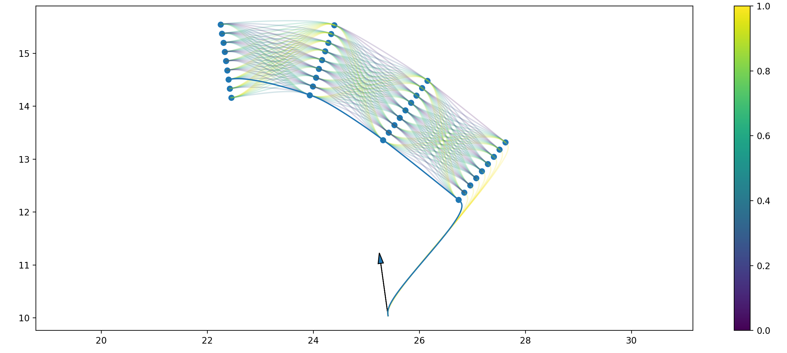
Fig. 1.3 Example Node Skeleton of Local Motion Planning. All Points of the different Layers are visualized and the correspending possible combinations of points, the resulting path between those and their respective cost visualized with the color map.
Altough we now know where we want to drive, the vehicle will not magically drive there :(.
Although we have had the idea for years to implement a remote control using an XBox controller to make the car drive “magically” by itself for years now :) Although, for the competitions this is of course a big no-no, so we sadly have to do this the hard way :(
—Martina Scheffler
We need one last module: The Control module uses a MPC with a linear bicycle model without tire and side forces as plant model and the planned trajectory as set value sequence. The output includes the optimal steering wheel angles and motor torques for the prediction horizon. One advantage of a MPC is that you are able to choose any predicted control input of the prediction horizon for the low-level controllers (torque controller, brake pressure controller and steering wheel angle controller).
The chosen steering wheel angle value is directly send to the steering actuator control PCB. The chosen torque, depending on the sign, is either converted to a necessary motor torque or brake pressure. The necessary motor torque is send to the vehicle control unit which delays the message to the inverter. The necessary brake pressure is further converted to a pneumatic brake pressure. This pressure is send to the ASBC, which controls the service brake valve. This resulting pneumatic pressure actuates the transducer, which leads to hydraulic brake pressure.
The Autonomous System now knows where it is, where the track is, what the optimal trajectory is and what the vehicle should do to follow this trajectory. We are finally driving. Well at least if everything is running smoothly. Welp.
Driving is almost always a success in itself. If you have made it to the point where the car starts accelerating, steering and braking by itself, count yourself lucky - even if it does not follow the track at first- and do not let other people tell you otherwise!
—Martina Scheffler